Notes on transmission lines
I mainly follow Pozar’s book
Lumped circuits and transmission lines
- When the electrical size of a circuit is negligible ($L/(c_1\omega)\ll 1$, with $c_1$ the speed of light in the wires) we can use the lumped circuit theory: circuits are made of voltage/current sources, resistors, capacitors, inductors, etc.
- Otherwise, the finite propagation speed of signals on wires must be taken into account. Transmission line theory must be used: voltage $v(z,t)$ and current $i(z,t)$ on cables are not only functions of time, but also of position.
Telegrapher’s model
Lines have an impedance per unit length: resistance $R$ and inductance $L$ in series, conductance $G$ and capacitance $C$ in parallel:
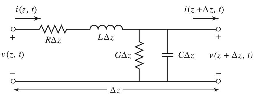
In a differential length, the telegrapher’s equations read:
\[\frac{\partial v}{\partial z} = -Ri - L\frac{\partial i}{\partial t}; \quad \frac{\partial i}{\partial z} = -Gv - C\frac{\partial v}{\partial t}\]In frequency domain, we define the complex phasors $V$(z) and $I(z)$ with $v(z,t)=\Re[V(z)\exp(-j\omega t)]$:
\[\frac{d V}{d z} = (-R+j\omega L)I; \quad \frac{d I}{d z} = (-G+j\omega C)V\]Caution: book uses $\exp(+j\omega t)$ instead.
We eliminate $I$ and introduce the complex propagation constant:
\(\frac{d^2 V}{dz^2} - \gamma^2 V = 0; \quad \gamma=\sqrt{(R-j\omega L)(G-j\omega C)} = j\omega\sqrt{LC}\beta\) with: \(\beta = \sqrt{\left(1+\frac{jR}{\omega L}\right)\left(1+\frac{jG}{\omega C}\right)} = \sqrt{\left(1-\frac{RG}{\omega^2 LC}\right) + j\left(\frac{R}{\omega L}+\frac{G}{\omega C}\right)} \simeq 1\)
The general solution is the sum of two traveling waves, one right and one left: \(V(z) = V_0^+\exp(+\gamma z) + V_0^-\exp(-\gamma z) = V^+(z) + V^-(z)\)
- $V_0^+$ and $V_0^-$ are the (initial) complex amplitudes of the voltage waves
- The imaginary part $\Im(\gamma)=k>0$ is the wavenumber of the propagating waves, and $\lambda =2\pi/k$ is the wavelength. The phase velocity satisfies $c_1=\omega/k$
- The real part $\Re(\gamma)=-\alpha<0$ gives the attenuation constant
We can write:
\[v(z,t) = V_0^+\exp(-j\omega t +jkz -\alpha z) + V_0^-\exp(-j\omega t -jkz +\alpha z)\]It is easy to check that the current follows an analogous equation
\[\frac{d^2 I}{dz^2} - \gamma^2 I = 0; \quad I(z) = I_0^+\exp(+\gamma z) + I_0^-\exp(-\gamma z)\]Using the first order equations we find that voltage and current complex amplitudes
\[V_0^+ = Z_0 I_0^+; \quad V_0^- = -Z_0 I_0^-;\]where we define the characteristic impedance of the transmission line as:
\[Z_0 = \sqrt{\frac{R-j\omega L}{G-j\omega C}} = \sqrt{\frac{L}{C}} \rho\]with
\[\rho = \sqrt{\frac{1+jR/(\omega L)}{1+jG/(\omega C)}} \simeq 1\]Ideal and real transmission lines
In an ideal transmission line $R$ and $G$ are zero, so
\[\gamma = ik = j\omega \sqrt{LC}; \quad \alpha = 0; \quad Z_0 = \sqrt{L/C}; \quad c_1 = 1/\sqrt{LC}\]In a real transmission line there is some attenuation $\alpha>0$, $Z_0$ is not purely real, and the phase velocity $c_1$ becomes weakly dependent on $\omega$
- Whenever $c_1$ is a function of $\omega$, there is dispersion
The parameters $L,C,R,G$ are geometry- and material-dependent. They also depend on the constants $\varepsilon_0$ and $\mu_0$
Read 2.2, ‘Field analysis of a transmission line’
Line termination
For an ideal line ($R,G=0$):
\(V(z) = V_0^+\exp(+jkz) + V_0^-\exp(-jkz)\) \(I(z) = \frac{V_0^+}{Z_0}\exp(+jkz) - \frac{V_0^-}{Z_0}\exp(-jkz)\)
The ratio between $V_0^+$ and $V_0^-$ on a transmision line depend on the termination load.
The load impedance fixes the ratio between $I$ and $V$ at the end of the line, where we place our origin $z=0$ for simplicity
\[Z_L = \frac{V(0)}{I(0)}\]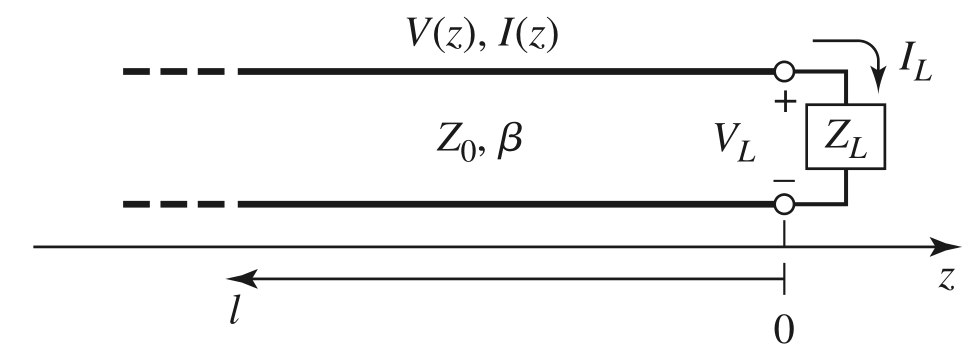
\[z=0 \Rightarrow \quad V(0) = V_0^+ + V_0^-; \quad I(0) = \frac{V_0^+}{Z_0} - \frac{V_0^-}{Z_0}\]
Hence:
\[Z_L = \frac{V(0)}{I(0)} = \frac{V_0^+ + V_0^-}{V_0^+ - V_0^-}Z_0 \quad \Rightarrow \quad V_0^- = \frac{V(0)}{I(0)} = \frac{Z_L - Z_0}{Z_L + Z_0}V_0^+\]-
We define the voltage reflection coefficient $\Gamma=V_0^-/V_0^+$, which is complex in general. The power reflection coefficient is $ \Gamma ^2$ - If $Z_L=Z_0$ there is no reflected wave and $\Gamma=0$. We say the load and the line are matched
- Any other situation leads to (partially) standing waves. The ratio between the maximum and minimum voltage in the line is the standing wave ratio SWR
The input of the line + load if the line has a total length $\ell$ is, by definition, the ratio between voltage and current at $z=-\ell$:
\[Z_{in} = \frac{V(-\ell)}{I(-\ell)}=\frac{1+\Gamma\exp(-2jk\ell)}{1-\Gamma\exp(-2jk\ell)}Z_0\]- For an unmatched line ($\Gamma\neq 0$), it is position-dependent
- If $\ell= n\lambda/2$, then $Z_{in}=Z_L$, regardless of $Z_0$
- If $\ell= \lambda/4+n\lambda/2$, then $Z_{in}=Z_0^2/Z_L$ (this is a so-called quarter-wave convertor)
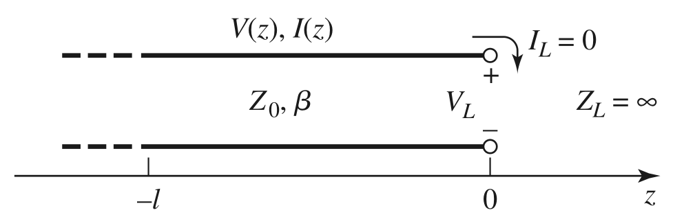
Open line
The load impedance is infinite, and $I(0)=0$ at the end of the line. This means that $\Gamma = 1$ and $Z_{in}=jZ_0 \tan(k\ell)$
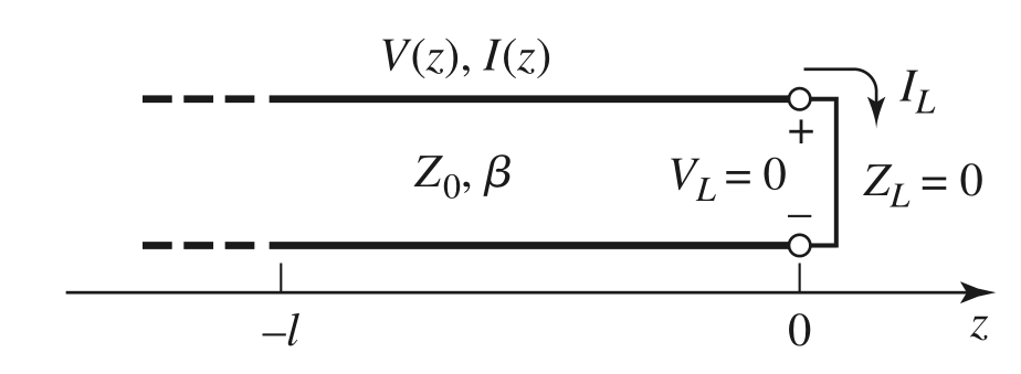
Shortcircuited line
The load impedance is zero, and $V(0)=0$ at the end of the line. This means that $\Gamma = -1$ and $Z_{in}=-jZ_0 \cot(k\ell)$
Discontinuity in characteristic impedance
Consider that we join two lines with $Z_0$ and $Z_1$ characteristic impedances. We assume a wave $V_0^+$ arriving from the left and a wave $V_1^-$ arriving from the right.
Equating voltages, currents at $z=0$:
\[V_0^+ + V_0^- = V_1^+ + V_1^-; \quad \frac{V_0^+}{Z_0} - \frac{V_0^-}{Z_0} = \frac{V_1^+}{Z_1} - \frac{V_1^-}{Z_1}\]We have 4 variables and 2 equations. We can compute $V_0^-$ and $V_1^+$ as the sum of a reflected and a transmitted wave:
\[V_0^- = \frac{Z_1-Z_0}{Z_1+Z_0}V_0^+ + \frac{2Z_0}{Z_1+Z_0}V_1^-; \quad V_1^+ = \frac{Z_0-Z_1}{Z_1+Z_0}V_1^- + \frac{2Z_1}{Z_1+Z_0}V_0^+\]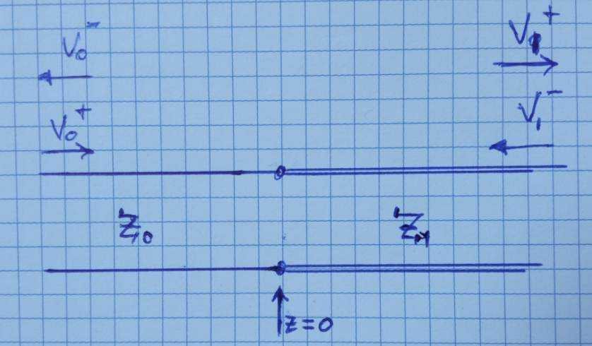
Looking from the left:
- The reflection and transmission coefficients are defined as
\(\Gamma = (Z_1-Z_0)/(Z_1+Z_0)\) \(T=2Z_1/(Z_1+Z_0)\)
- The insertion loss is $T$ in dB
Power conservation takes the form: \(1/Z_0 = \Gamma^2/Z_0 + T^2/Z_1\)
Interlude: decibels
Any energy or power ratio $P_1/P_2$ can be expressed in dB as
\[10 \log_{10} \frac{P_1}{P_2} \,\, \text{dB}\]Since powers are the squares of amplitudes (e.g. voltages or currents), we can also express amplitude ratios such as $V_2/V_1$ in dB with
\[20 \log_{10} \frac{V_1}{V_2} \,\, \text{dB}\]Electrical engineers like expressing not just ratios, but absolute quantities refered to e.g. 1 mW (for power), 1 V (for voltage), etc. Then we write:
\(10 \log_{10} P_1 (\text{in mW}) \,\, \text{dBmW}\) \(20 \log_{10} V_1 (\text{in V}) \,\, \text{dBV}\)
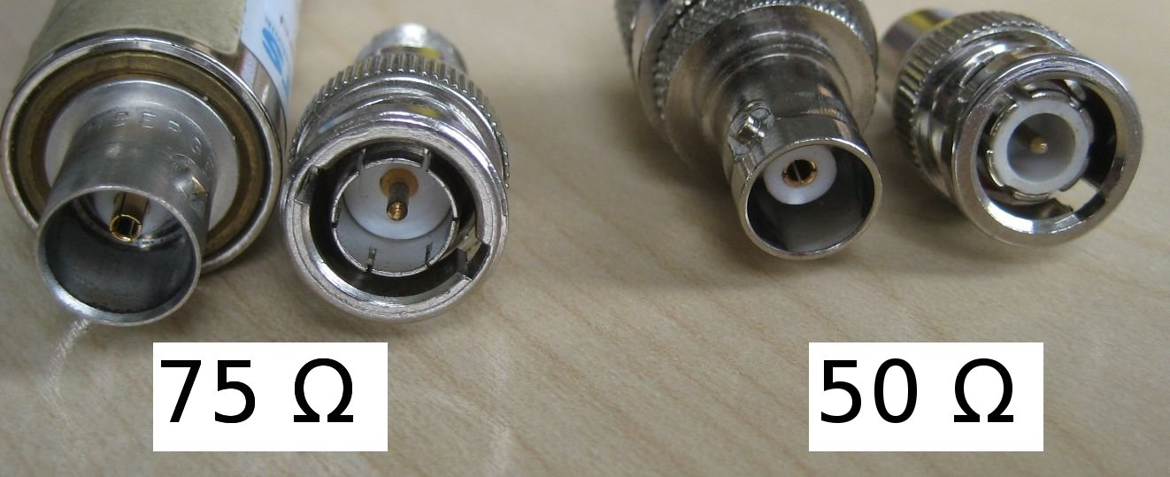
Common coaxial connectors
BNC: bigger. Female/male. Quarter turn to mate. Up to 2 GHz roughly. Common variants exist for 50 or 75 Ohm lines. Typically, male connector is on the cable, female connector on the equipment. High voltage alternatives: MHV, SHV
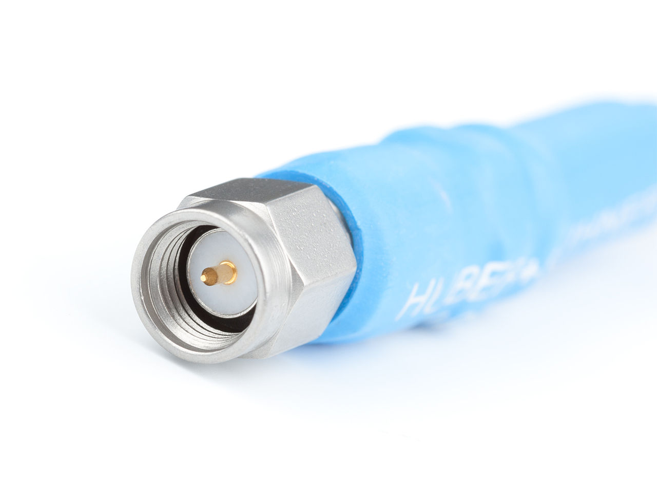
SMA: smaller. Female/male. Threaded. Up to several GHz and very common in microwave systems. 50 Ohm.
N connector: common for power applications
Balanced - unbalanced transmission lines
Transmission lines discussed so far are of the “unbalanced” type: the signal wire and the ground wire in the cable are physically different and serve different roles (e.g. a coaxial cable).
If the two wires are identical, they both have opposite voltage and current at each point. This is a “balanced” line, where both leads may float with respect to ground. Optionally, there may be a “shield” around the two wires playing the role of ground. This setup can be studied with two lines + ground line.
Side comment, partially related:
Observe that our transmission line model assumes a lumped ground with constant voltage everywhere. The real ground wire may exhibit varying voltage and current with distance.
Ground loops
A ground loop occurs whenever there are more than two paths to ground in a circuit. Since the wire ground loop usually has very low resistance, often below one ohm, even weak external magnetic fields can induce significant currents.
The alternating ground current flowing through the cable can introduce AC voltage drops due to the resistance, and therefore interferences.
Ground currents through the shield of a coaxial also create noise on the signal and voltage differences among the various grounds. Ground currents can be induced by external oscillating B fields or by an equipment that leaks to ground
Single-point grounding to the building and ``breaking’’ ground loops with transformers, etc, are techniques to reduce ground noise.