Notes on the basic two-fluid collisionless magnetoplasma model

Assumptions

These assumptions define the regime of validity of the model:

• Fully-ionized ion-electron plasma (we ignore neutrals).
• $\partial/\partial t = 0$: Steady-state plasma.
• $\lambda_D^2 = \varepsilon_0 T_e/(ne^2)\ll L^2$: quasineutral plasma $n=n_i=n_e$.
• $\chi_H = \omega_{ce}/\nu_e \gg 1$, $u_i/L\gg\nu_i$: Collisionless plasma.
• $\ell_e \ll L$: electrons are fully magnetized. We only keep zeroth-order terms in $\ell_e/L$.
• $m_e u_e^2 \ll T_e$: negligible electron inertia and bulk velocity.
• $m_i u_i^2 \sim T_e$: moderate bulk ion velocity.
• $T_i \ll T_e$: cold ions.
• $\beta = 2nT_e/(\mu_0 B^2)\ll 1$: negligible induced magnetic field.

Ion equations

Continuity: \(\nabla \cdot (n \bm u_i) = 0\)

Momentum: \(m_i \bm u_i \cdot \nabla \bm u_i = -e \nabla \phi + e \bm u_i \times \bm B\)

• Note this is the “non-conservative form.”
• Ion magnetic force is often neglected (unmagnetized ions). Note that $m_i\gg m_e$.
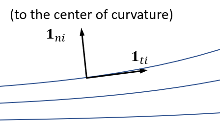
• Left-hand side can be expressed as ($\bm 1{t i}$, $\bm 1{n i}$ are the tangent and normal unit vectors to ion trajectories; $\kappa_i$ the ion trajectory curvature): \(m_i \bm u_i \cdot \nabla \bm u_i = \frac{1}{2}m_i \frac{\partial u_i^2}{\partial \bm 1_{t i}} \bm 1_{t i} + m_i u_i^2 \kappa_i\bm 1_{n i}\)

Projection along $\bm 1_{\parallel i}$ is integrable: \(\frac{1}{2}m_i u_i^2 + e\phi = H_i\)

• Mechanical energy equation.
• Valid along ion streamlines.

Electron equations

We write $\bm u_e = u_{\parallel e} \bm 1b + \bm u{\times e}$. We will call $\bm 1\times = \bm u{\times e} / u_{\times e}$, and $\bm 1\perp = \bm 1\times\times \bm 1b$. ${\bm 1_b,\bm 1\perp,\bm 1_\times}$ is a right-handed, orthonormal vector basis.

Continuity: \(\nabla \cdot (n \bm u_e) = 0 \\ \nabla \cdot(nu_{\parallel e} \bm 1_b + n\bm u_{\times e}) = 0\)

• This is the only electron equation where $u_{\parallel e}$ is present.

State: \(p_e = nT_e\)

• Isotropic electrons.

Momentum: \(\bm 0 = -\nabla p_e + en \nabla \phi - en \bm u_{\times e} \times \bm B\)

• Balance of pressure, electric, and magnetic forces.

If a barotropy function $h_e$ exists such that $\nabla h_e = (\nabla p_e)/n$, then: \(\bm 0 = -\nabla h_e + e\nabla \phi - e\bm u_{\times e} \times \bm B\)

• A barotropy function exists if the electrons are isothermal, $T_e=\text{const}$ and $\gamma=1$, or polytropic, $T_e\propto n^{\gamma-1}$: \(h_e = \gamma T_e \ln n\)
• This is known as a closure relation at the temperature level. Other models exist that use the energy equation and a closure relation at the heat flux level (they may not have a barotropy function).

Projection along $\bm 1b$ or along $\bm 1\times$ yields: \(0 = \bm 1 \cdot[-\nabla h_e + e\nabla \phi], \quad \text{where: } \bm 1= \bm 1_b,\bm 1_\times\)

• Balance of pressure and electric forces.

Integrating: \(h_e-e\phi = H_e\)

• Energy conservation equation.
• Valid along electron streamlines $=$ magnetic streamlines.
• Valid in the $\bm 1\times$ direction too: $\bm 1_b$ and $\bm 1\times$ define nested surfaces. We can call them $H_e$-surfaces.

We can re-write the momentum equation as: \(\nabla H_e = - e\bm u_{\times e} \times \bm B\)

• $\nabla H_e = (\nabla p_e)/n - e\nabla\phi$ is equal to the magnetic force per electron

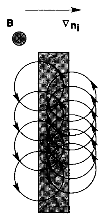
Crossing with $\bm B$ and operating: \(\bm u_{\times e} = \frac{\nabla H_e\times \bm B}{eB^2}\)

• Explicit expression for $u_{\times e}$, the Hall velocity, and $\bm 1_\times$, the Hall direction.
• $\bm u_{\times e}$ is the sum of the $\bm E\times\bm B$ drift and the diamagnetic drift $\nabla p_e \times \bm B / (enB^2$). This is not a particle drift, but a fluid drift due to the collective motion of the electrons.

Ion equations, revisited

• These are analogous to Euler gasdynamics equations for a polytropic species, with the extra force terms $\nabla H_e$ and $e \bm u_i \times \bm B$.

Important remarks

• Electron momentum equation is fully algebraic after applying the simplifying assumptions.
• Given $\bm B$ and boundary conditions, $H_e$, $u_{\times e}$, $\bm 1_\times$ are fully determined before computing anything else.
• The boundary conditions must set one and only one value of $H_e$ on each magnetic line (else they are incomplete or incompatible).
• Once $H_e$ is known, we can integrate the ion differential equations, finding $n$, $\bm u_i$.
• Once $n$ is known, the electron continuity equation can be used to compute $u_{\parallel e}$.
• Once $n$ and $H_e$ are known, from closure relation and the state equation we can compute $p_e$, $T_e$.
• Finally, from the conservation of $H_e$ we can compute $\phi$.

Model extensions

Assumptions can be relaxed, but the model complexity increases accordingly:

• Adding collisions allows electrons to move in the $\bm 1\perp$ direction. Also, $u{\parallel e}$ now appears in the momentum equation.
• Adding ionization/recombination: source terms in the ion and electron equations.
• Interactions with walls: non-neutral sheath models can be employed.
• Time dependence: all differential equations become fully hyperbolic then.
• Replace isothermal/polytropic closure with electron energy equation plus a higher-order closure.
• Include heating term in energy equation (e.g. EM power deposition).
• Extend the temperature model to include electron anisotropy.
• Include ion temperature.
• Include the plasma-induced magnetic field through Ampère’s equation.